Meteorology unit 1

Since learning to fly my interest has broadened from exploring the mountains to understanding the air. I am now studying meteorology, which is giving a physical and mathematical background to some of the concepts I have learnt, as well as introducing some new ideas. Meteorology can get complex pretty quickly, so it’s hard to know where to start. I’ll try to focus on a few different maps and charts that illustrate a few principles that I found interesting in the introductory part of the course. It’s not necessarily well organised or explained so don’t expect to understand it all in a single reading… but hopefully it provides some insight into what is meteorology is about.

Himawari satellite viewer

Note: where possible I’ve added links to the source of images.

Our atmosphere

There are a few special things which make earth a place where we can live.

Earth’s atmosphere from space

Firstly, understand that the atmosphere is incredibly thin.

If the surface of earth was a sheet of A4 paper, the thickness of the paper is equal to the height of Everest. More than two thirds of the atmosphere by mass lies below it.

Although it’s all air, different things happen in different parts of the atmosphere. Much of it crucial for life on earth.

• In the thermosphere, earth’s magnetic field protects us from the solar wind and acts to stop the atmosphere fizzing out into space. The ionosphere is in this region.
• A tiny amount (if brought to sea level only 2-3 millimetres thick) of ozone protects us from ultraviolet (UV) radiation. 2% of suns energy is UV
• The warming above the tropopause (between troposphere and stratosphere) caps storms and cyclones, preventing them building up until they reach space

Know that:

• The pressure is just a measure of the weight of the air on top. 1000hPa (=1000 millibars) is equal to ten tons of air over each square metre. Since water is one ton per cubic metre, one metre underwater the pressure increases by 10%.
• Most gases are evenly mixed throughout, up to the mesosphere (nitrogen 78%, oxygen 21%, other gases 1% including 0.04% carbon dioxide), but ozone is in the stratosphere, and water vapour almost all in the troposphere
  

  Greenhouse gas distribution in the atmosphere (average only!!)

• Water vapour is an invisible gas. Cold air holds exponentially less. This is why clouds (or condensation on a cold beer) form…

Warm air can hold (way!) more water vapour

The greenhouse effect is a blanket that helps moderate temperatures on earth. Due to the greenhouse effect:

• the earth is around 30°C warmer overall.
• The coldest nights are when you are high in arid regions with clear sky (very little water vapour in the air to slow cooling)
• Even a thin layer of cloud acts like a “blanket”

The ozone destroying chemical CFC banned in the 1990’s is a potent greenhouse gas but of relatively low concentration. Similarly for methane. Water vapour is in fact the most significant greenhouse gas, but unlike carbon dioxide it only lasts for several days in the atmosphere and is of highly variable concentration (mostly near the surface).

The sun

The sun provides the energy for weather. Understanding and modelling weather is all about how the energy from the sun interacts with the earth.

Energy from the sun in watts per square meter averaged over a day

Before interacting with the atmosphere the sun provides 1361 watts per square. This is averaged out over the whole surface of the earth (which is 4x the area of the disc) to give average incoming solar radiation (insolation) values in the graph above. This graph is energy received at the top of the atmosphere so it excludes reflections from clouds, etc. The maximum is near the South Pole because it has 24hour sunlight in austral summer when earth is slightly closer to the sun. Otherwise it’s highest in the tropics.

Energy reaching earth (blue sky)

The sun emits all kinds of radiation but the highest intensity is visible light. In a cloud free atmosphere most of suns energy reaches earth. The atmosphere scatters some wavelengths (for example blue light, giving the sky colour) and absorbs others (for example greenhouse gases absorbing heat).

Scattering regimes depend on the ratio of ray wavelength to particle size

• Geometric optics are where refraction takes place inside water droplets or ice crystals, examples are rainbows, haloes, sun dogs, pillars, coronas, iridescence, circumzenithal arc…
• Mie scattering is mostly back in the direction it came from so weather radars are designed around wavelengths that detect raindrops (microwave)
• Rayleigh scattering is in all directions, and it is highly wavelength dependent so blue light is scattered a lot more than red light, giving the sky colour

Circumzenithal arc above halo, taken in the Southern Ocean, 16/11/13

A theoretical black body absorbs all radiation and re-emits at a rate dependent on its temperature. The spectral irradiance curve above from the sun is approximately black body for a surface of around 5500°C. Most surfaces on earth are approximately black body too, and making that assumption we determine brightness temperature of the surface simply by measuring the intensity at a given wavelength.

X-rays, UV, Light, thermal IR, microwaves, and radio waves are all in the electromagnetic spectrum. The thing which makes them different to each other is their wavelength / frequency. We refer to solar wavelengths such as visible light as shortwave (SW) and thermal IR as longwave (LW).

• Radio waves – about four times the length of your antenna
• Radar (microwave) 5-10cm,
• Thermal IR 4-100µm, (1000,000µm = 1m)
• at 4µm, 99% of suns radiation is on the SW side and 99% of the earths outgoing radiation (excluding reflections) is on the LW side
• Near IR 0.76-4µm
• Visible 0.39-0.76µm,
• UV 0.2-0.39µm
• X-rays and Gamma rays (shortest wavelength)

The electromagnetic spectrum

Solar heating

Earths energy budget

The oceans cover 71% of the surface. Sun shines deep into the water and waves distribute the heat through a hundred metres or so, reducing daily temperature variations. In fact the  oceans are warmest about two months after the maximum summer heating. Since temperature variation is minimal, thermals are weak and usually under 1km high.

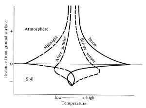
Daily surface heating

The land only heats through about 5-10cm depth, depending on the surface. In dry areas all suns energy can be converted into sensible heat (temperature change) rather than latent heat (evaporating water). This results in intense thermals that can reach as high as 3km in the summer. This variable depth of atmosphere above the surface is the planetary boundary layer.

Vertical temperature profiles

The red graph shows how hot you would need to heat air for outgoing radiation to balance insolation, if there were no thermals or evaporation (conduction within air is negligible anyway). This would result in a very unstable atmosphere (surface about 55°C +273.15=328K).

If dry air thermals are introduced, mixing from convection changes the graph to follow the dotted line, with cooling at about 10°C/km (dry adiabatic lapse rate). This would mean we could ride thermals up to the tropopause, which just doesn’t happen on blue sky days.

In practice, above the boundary later the lapse rate is closer to 6.5°C/km. Generally we don’t have to lift air very high for it to cool to dew point, and clouds form. When clouds are forming they release latent heat so the cooling rate reduces. When air subsides again it warms at 10°C/km, but over several days to weeks the heat is lost through radiation.

Earth cooling

Since the sun is shining straight at it, the tropics are hotter than the poles. This is the driving force behind the global circulation, a wind regime that helps redistribute heat. If not for this heat transport the tropics would be even hotter, and the poles even colder.

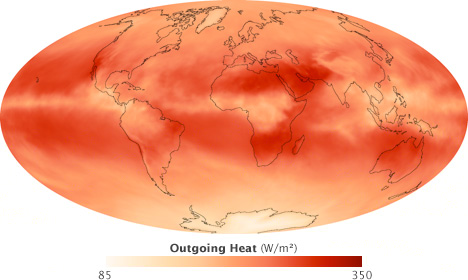
Outgoing heat in September 2008 (NASA)

This graph shows outgoing heat measured by a satellite and averaged over time. It is colder nearer the poles and in areas that are typically cloudy, since the cloud tops are cold. You can notice the lighter shading around the tropics.

Instantaneous outgoing heat values for black bodies (most surfaces approximate this):

• A surface at -30°C radiates 200 watts per square metre
• A surface at -3°C radiates 300 watts per square metre
• A surface at 17°C radiates 400 watts per square metre
• A surface at 33°C radiates 500 watts per square metre

Some of this energy is absorbed by the atmosphere and reflected back to earth, particularly if there is cloud which is a very good absorber.

The red bands of outgoing heat are hottest because they are close to the tropics, and they are in relatively cloud free areas – the subtropical high pressure belts. More on this next.

Global circulation

The surface winds and upper return flows, averaged over a year, are approximated by the Hadley circulation model.

Global Hadley circulation

The uneven distribution of heating creates differences in air densities resulting in pressure gradient force (PGF) from high pressure to low. After a few hours wind begins to feel Coriolis force (CoF) due to earth’s rotation, acting to the left of the wind in the southern hemisphere. Geostrophic wind is a balance between CoF and PGF, with the wind at right angles to both. In the southern hemisphere put your right thumb up for a high pressure system and the geostrophic wind will rotate in the direction of your fingers. In the real world friction tends to reduce wind speeds by about 30% over sea and say 70% over land, which reduces CoF (proportionally to wind speed) and results in wind tending to flow a little outwards from highs and slightly inwards into lows.

Thickness, thermal wind shear, and geostrophic wind

A column of the atmosphere, if heated, will expand (the Ideal gas law says if you cool an empty bottle from 30°C=300K to 270K=freezing it will shrink by 10%). A heated column will therefore be higher than its cooler surroundings and air will spill out the top. Eventually the air will be subject to CoF and the wind will blow with warm air to the left (in the southern hemisphere). This thermal wind shear means that on average, winds tend to the west at altitude (in both hemispheres), because it is warmer toward the equator. A consequence of this (that I won’t try and explain here) is that if air veers with altitude it is bringing in colder air (cold air advection) and if it backs we have warm air advection (opposite in the northern hemisphere). The thermal wind helps explain why we have the jet stream, and why the jet stream is strongest up at the tropopause.

Aside from CoF and PGF, there are other balanced winds. Gradient wind is similar to geostrophic with the added consideration of centrifugal force (CeF). On a small scale where Coriolis is weak, CeF can oppose PGF for cyclostrophic balance in either direction around a Low. A seabreeze has an inertial turning as it is acted on by CoF balancing CeF. Also in the direction of the wind the seabreeze has antitriptic balance between the weak PGF and surface friction.

Thickness / MSLP chart, indicating a cold dense airmass extending into SE Australia

The inter tropical convergence zone (ITCZ) migrates with the seasons, bringing the monsoon with it. Monsoon is a deep westerly wind with an onset, several break periods of weekly timescales, and retreat. Monsoon brings humid air across the equator causing increased storm and cyclonic activity. While the Hadley circulation implies ascent in the ITCZ, we are told that the typical state is cloud free subsidence – it is the short lived thunderstorms and cyclones which upset the average.

One thing that never occurred to me is that cloud top cooling (particularly at night) is a significant contributor to instability and overturning within large clouds (only the top surface cools as the rest keeps itself warm). This can result in thunderstorms during the night.

In the tropics (loosely between 23.5°N and 23.5°S depending on context), CoF is weak and the corresponding PGF is also weak. Since there is very little pressure difference driving winds the weather is more subtle and harder to predict. Hot and humid conditions mean that often the dominant force in the tropics is latent heat, the driving force behind thunderstorms and cyclones. Large scale convergences between different circulation patterns increase the chances that something will start to develop. Trade winds feed into the ITCZ (southeast in the southern hemisphere) and the monsoon brings wind from the opposite direction.

In the mid-latitudes pressure gradients dominate and familiar High and Low pressure systems are the dominant influence on weather. The jet stream winds and the associated forces interacting with CoF move the upper air mass around, causing development of surface features. For example, at the exit of a jet stream the sudden deceleration steers the flow toward the equator, favourable for surface low development on the poleward side. Highs and lows are cyclical in nature with the associated Rossby waves typically oscillating over a week or so. Now that we are ingesting satellite data, Numerical Weather Prediction (NWP) models are quite good at predicting surface pressure in the mid-latitudes over timescales of about a week.

Forecast model accuracy improvement over the years

I am told that greater ingestion of satellite data into the NWP models is largely attibutable to increased performance, however it is also true that increased supercomputer performance has facilitated this.

The temperature trace (sounding)

The trace is also known as a skew-T plot, sounding, an F160 (within BOM), or tephigram (slightly different). It is one of the most important tools for a forecaster, giving a snapshot of the atmosphere over a point. It is measured daily with balloon flights throughout the world and by selected commercial aircraft.

There is also a clever method that deduces temperature profiles using satellite data and the known absorption characteristics of certain well mixed gases (such as CO2) at certain exact wavelengths with reasonable accuracy (there is huge scope for improved satellite instrumentation here).

Temperature trace in Antarctic winter

To the unfamiliar it looks like a bit of a mess of lines – I’d suggest spending some time reading about them. The image below is from Vertical Stability on the BOM aviation website.

With the exception of airmass boundaries like fronts or sea breezes, the atmosphere away from the surface changes only very gradually in the horizontal direction. The vertical direction on the other hand is highly variable. This is facilitated because only small imbalances in the horizontal are equalised by wind, but in the vertical direction hydrostatic forces (pressure vs gravity) are orders of magnitude higher than any other meteorological forces.

Also any vertical motion results in expansion / contraction to match the surrounding pressure which results in significant changes in temperature. In general the atmosphere is quite stable so it resists these motions. However, while small, vertical motion is fundamentally crucial to our weather, and this is why the temp trace is so important.

BOM trace explanation

As complicated as this chart is, it saves a great deal of horrendous and highly mathematical thermodynamic physics. The 9 assumptions of parcel theory give us a very good approximation for what actually happens. There are a few related points I’ll mention but won’t explain:

• With a vague idea of the synoptic situation, often one can be pretty precise about what will happen by looking at the stability and moisture, and estimating insolation energy (translating to area on the chart)
• The chart does not tell us about air in thermals mixing with its surroundings (entrainment), momentum or drag, and ignores cloud droplets once they’ve formed.
  

  Some assumptions we make with the temp trace

• We also often ignore humidity for buoyancy. To be precise, a humid parcel has the same buoyancy as a dry parcel raised to a virtual temperature, Tv = T + r/6. As an example, sea level 21°C 75%RH air has Tv=23°C.
• A well mixed layer will have temperature along the adiabat (dry or wet as appropriate), and constant mixing ratio. Before mixing it will have equal areas above and below these lines. The boundary layer is the layer of variable thickness that is in contact with the earth, its size is related to instability and solar heating.
  

  Mixing can create inversions

• As a rule of thumb,
  • “low” cloud is warm water droplets (above 0°C),
  • mid level such as altostratus or altocumulus is supercooled water, and
  • high level where ice starts to form is below -20°C. This icing needs to be reached for cumulonimbus development, the only cloud which can produce thunderstorms.
• Latent instability relates to whether a lifted parcel will ever reach a level of free convection (LFC) where it becomes warmer than the environment and continues rising to the equilibrium level (EL). The energy required for lifting is the convective inhibition (CIN) and the energy released above LCL is the convective available potential energy (CAPE) for thunderstorms.
  

  Forecasting thunderstorm development

  

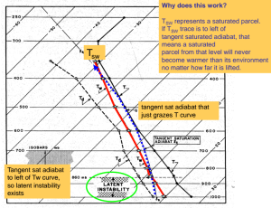
  Latent instability

• Potential instability relates to whether a layer will become unstable if the whole airmass is lifted (for example, by a cold front). The wet bulb trace is used to determine this and the outcome is that with moisture even large inversions can be overcome very quickly.
  

  Wet bulb temperature

• Due to the thermal wind shear, with altitude the wind tends to the west and increases. Veering with altitude suggests cold air advection (CAA) into the layer and backing WAA (opposite in the northern hemisphere). Differentials between CAA and WAA in different layers effects stability.

Satellite observations

Satellites have revolutionised meteorology. The two most common orbits are low earth orbit (LEO) which complete a revolution in around two hours, and geostationary (GEO) which orbit in sync with earths rotation, maintaining their position above the same point on the equator. In late 2014 Japan provided us with a significant upgrade to GEO imagery with the Himawari 8. Unlike LEO, GEO satellites are high enough to see the full disk of the earth. With images every ten minutes from the same location above earth, we can see the movement of weather systems and get a real insight into the dynamics as shown in the moving cloud patterns. Check it out! 

The BOM day / night product

Some ways we use satellites:

• VIS for high definition images showing cloud shadows, overshooting tops in thunderstorms, fog, smoke… all only during daylight, and always comparing with IR
• IR for brightness temperature, most commonly checking the temperatures (height) of cloud tops
• NIR (near IR) for comparing with the IR to help identify fog
• WV (water vapour) for seeing the mid and upper atmosphere (there is too much water vapour lower down so we can’t see “through” to that level)
• ASCAT winds, for identifying surface winds over ocean based on wave heights
• CIMSS winds, for identifying winds at different heights based on opportunistic cloud drift measurements. Archived with other imagery

Hear more from the master, one of our most enthusiastic and knowledgable lecturers:

Forecasting

As you can see there is certainly a lot of information to consider when preparing a forecast, so it helps to have a clear forecast process. First we zoom out and look at the overall situation and the events leading up to it, and look at how well our models are representing the current situation. Later we begin to zoom in and make fine adjustments considering local area effects. The meteorology course involves a lot of physics and mathematics but this will be left to the computers so it’s appropriate that there is an emphasis on developing a conceptual understanding. I have good micrometeorology understanding from flying but it’s also been interesting learning about the upper atmosphere.

Where do I get forecasts when travelling the world? For me something that explains the overall situation then gives specific details about different altitudes, like the Chamonix forecast would be ideal, or in New Zealand the basic Southern Lakes forecast gives you a general idea, but it’s not always that get a forecast with the information you need. The basic principle is that you want to be familiar with what you are looking at, which is why I often try to find a synoptic chart. Often I have poor internet if at all so frequently I just resort to asking passers by. The main problem is that the public weather forecasts concern one point on the surface, whereas for aviation you are concerned with multiple levels over a larger area. If you have good internet, combining windyty with forecasted GFS soundings gives you plenty of data to play with. And remember… it’s only a forecast!

Windyty (amazing visualisation of the GFS* model forecast) *EC recently added

More info: check the Antarctic Forecasting Handbook